
One big challenge that faces casualty insurance companies is that they tend to be overwhelmed by the amount of claims. To streamline the workload, it would be desirable if the claims can be prioritized in some ways. In the case of automobile accidents, the claim adjuster would probably like to know the potential loss based on the make and model of the vehicles and prioritize his cases on that metric.
In this blog, we are going to use a dataset from UCI. The main goal here is to illustrate a powerful feature called pipeline in Python’s Scikit Learn library where you can transform data on the fly while training your machine learning model. You may have noticed that the term pipeline is used extensively in machine learning. It may mean very different things when used elsewhere! But in this context, we’re using it to refer to pipeline objects in Scikit-Learn.
The data set and pertinent information can be found in the link below and will be not repeated here. Please read the description of the data set and refer to it when necessary.
https://archive.ics.uci.edu/ml/datasets/automobile
The original data file imports-85.data is comma delimited. So the extension was changed, column headings added and extension changed to csv. Rows with missing values in the “normalized-losses” column were removed and the file was renamed to AutoInsuranceClaimNoMissingLoss.csv for training the model.
#Import modules we'll need for this exercise
import pandas as pd
from sklearn.ensemble import GradientBoostingRegressor, RandomForestRegressor
from sklearn.metrics import mean_squared_error, r2_score
from sklearn.model_selection import train_test_split
import numpy as np
import matplotlib.pyplot as plt

#Load and train data set
claim_data = pd.read_csv("c:/doc/AutoInsuranceClaimNoMissingLoss - 3_31_22.csv")
claim_data.head()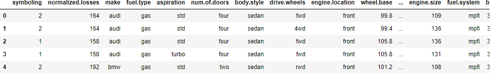
Examine the data types in the data frame.
claim_data.dtypes
symboling              int64
normalized.losses      int64
make                  object
fuel.type             object
aspiration            object
num.of.doors          object
body.style            object
drive.wheels          object
engine.location       object
wheel.base           float64
length               float64
width                float64
height               float64
curb.weight            int64
engine.type           object
num.of.cylinders      object
engine.size            int64
fuel.system           object
bore                 float64
stroke               float64
compression.ratio    float64
horsepower             int64
peak.rpm               int64
city.mpg               int64
highway.mpg            int64
price                  int64
dtype: object
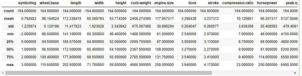
Identify the numerical features and categorical features and look at the statistics of the numerical features.
numeric_features = ['symboling','wheel.base','length','width','height','curb.weight','engine.size','bore','stroke','compression.ratio','horsepower','peak.rpm','city.mpg','highway.mpg','price']
categorical_features = ['make',	'fuel.type','aspiration','num.of.doors','body.style','drive.wheels','engine.location','engine.type','num.of.cylinders','fuel.system']
claim_data[numeric_features + ['normalized.losses']].describe().of.cylinders','fuel.system']claim_data[numeric_features + ['normalized.losses']].describe()

Notice that columns bore and stroke have 0’s. According to the document, bore should have values from 2.54 to 3.94 and stroke should have values from 2.07 to 4.17. We will replace 0 with the mean of the feature.
bore_mean=claim_data[claim_data["bore"] != 0]["bore"].mean()
claim_data['bore'] = np.where(claim_data['bore'].eq(0),bore_mean,claim_data['bore'])
stroke_mean=claim_data[claim_data["stroke"] != 0]["stroke"].mean()
claim_data['stroke'] = np.where(claim_data['stroke'].eq(0),stroke_mean,claim_data['stroke'])
claim_data[numeric_features + ['normalized.losses']].describe()
# Separate features and labels
# After separating the dataset, we now have numpy arrays named **X** containing the features, and **y** containing the labels.

X, y = claim_data[numeric_features + categorical_features ].values, claim_data['normalized.losses'].values

# Split data 70%-30% into training set and test set
X_train, X_test, y_train, y_test = train_test_split(X, y, test_size=0.30, random_state=0)

print ('Training Set: %d rows\nTest Set: %d rows' % (X_train.shape[0], X_test.shape[0]))
Training Set: 114 rows
Test Set: 50 rows
So far, we are looking at the data that is virtually loaded straight from a source file with only a little preprocessing.
In practice, it’s common to perform much more preprocessing of the data to make it easier for the algorithm to fit a model to it. There’s a huge range of preprocessing transformations you can perform to get your data ready for modeling. In fact according to surveys, data scientists spend about 80% of their time organizing data, doing feature engineering and preprocessing transformations of data. But we’ll limit ourselves to a few common techniques for this short demo of how pipeline works.
Scaling numeric features
Normalizing numeric features so they’re on the same scale is important. It prevents features with large values from producing coefficients that disproportionately affect the predictions. When all features are in the same scale, it also helps algorithms to understand the relative relationship better.
There are multiple ways you can scale numeric data, such as calculating the minimum and maximum values for each column and assigning a proportional value between 0 and 1, or by using the mean and standard deviation of a normally distributed variable to maintain the same spread of values on a different scale.
More info can be found in the link below.
https://www.kdnuggets.com/2020/09/feature-engineering-numerical-data.html
Encoding categorical variables
Many machine learning models do not work with text values. Therefore, you generally need to convert categorical features into numeric representations. There are many ways to encode text values to numerical values, such as ordinal encoding which substitutes a unique integer value for each category, and one hot encoding that creates individual binary (0 or 1) features for each possible category value.
You can learn more about it in the following link.
https://www.kdnuggets.com/2019/07/categorical-features-machine-learning.html
To apply these preprocessing transformations to the insurance claims data, we’ll make use of a Scikit-Learn feature called pipelines. These enable us to define a set of preprocessing steps that end with an algorithm. You can then fit the entire pipeline to the data, so that the model encapsulates all of the preprocessing steps as well as the regression algorithm. This is useful, because when we want to use the model to predict values from new data, we need to apply the same transformations (based on the same statistical distributions and category encodings used with the training data).
# Train the model
from sklearn.compose import ColumnTransformer
from sklearn.pipeline import Pipeline
from sklearn.impute import SimpleImputer
from sklearn.preprocessing import StandardScaler, OneHotEncoder

# Train the model
from sklearn.ensemble import GradientBoostingRegressor, RandomForestRegressor

import numpy as np

# Define preprocessing for numeric columns (scale them)
numeric_features = [0,1,2,3,4,5,6,7,8,9,1,11,12,13]
numeric_transformer = Pipeline(steps=[
    ('scaler', StandardScaler())])

# Define preprocessing for categorical features (encode them)
categorical_features = [14,15,16,17,18,19,20,21,22,23]
categorical_transformer = Pipeline(steps=[
    ('onehot', OneHotEncoder(handle_unknown='ignore'))])

# Combine preprocessing steps
preprocessor = ColumnTransformer(
    transformers=[
        ('num', numeric_transformer, numeric_features),
        ('cat', categorical_transformer, categorical_features)])

# Create preprocessing and training pipeline
pipeline = Pipeline(steps=[('preprocessor', preprocessor),
                           ('regressor', GradientBoostingRegressor())])


# fit the pipeline to train a linear regression model on the training set
model = pipeline.fit(X_train, (y_train))
print (model)
Pipeline(steps=[('preprocessor',
                 ColumnTransformer(transformers=[('num',
                                                  Pipeline(steps=[('scaler',
                                                                   StandardScaler())]),
                                                  [0, 1, 2, 3, 4, 5, 6, 7, 8, 9,
                                                   1, 11, 12, 13]),
                                                 ('cat',
                                                  Pipeline(steps=[('onehot',
                                                                   OneHotEncoder(handle_unknown='ignore'))]),
                                                  [14, 15, 16, 17, 18, 19, 20,
                                                   21, 22, 23])])),
                ('regressor', GradientBoostingRegressor())])
The model is trained with GradientBoostingRegressor, including the preprocessing steps. The following code shows how it performs with the validation data.
# Get predictions
predictions = model.predict(X_test)

# Display metrics
mse = mean_squared_error(y_test, predictions)
print("MSE:", mse)
rmse = np.sqrt(mse)
print("RMSE:", rmse)
r2 = r2_score(y_test, predictions)
print("R2:", r2)

# Plot predicted vs actual
plt.scatter(y_test, predictions)
plt.xlabel('Actual Labels')
plt.ylabel('Predicted Labels')
plt.title('Insurance Claim Predictions')
z = np.polyfit(y_test, predictions, 1)
p = np.poly1d(z)
plt.plot(y_test,p(y_test), color='magenta')
plt.show()
MSE: 266.7675806643773
RMSE: 16.3330211738177
R2: 0.7351873720799795

The final pipeline is composed of two pipelines that do the transformations (preprocessor) and the algorithm used to train the model. To try an alternative algorithm you can just change the final pipeline to include a different kind of estimator. Code example below shows that the final pipeline uses the RandomForestRegressor.
# Use a different estimator in the pipeline
pipeline = Pipeline(steps=[('preprocessor', preprocessor),
                           ('regressor', RandomForestRegressor())])


# fit the pipeline to train a linear regression model on the training set
model = pipeline.fit(X_train, (y_train))
print (model, "\n")

# Get predictions
predictions = model.predict(X_test)

# Display metrics
mse = mean_squared_error(y_test, predictions)
print("MSE:", mse)
rmse = np.sqrt(mse)
print("RMSE:", rmse)
r2 = r2_score(y_test, predictions)
print("R2:", r2)

# Plot predicted vs actual
plt.scatter(y_test, predictions)
plt.xlabel('Actual Labels')
plt.ylabel('Predicted Labels')
plt.title('nsurance Claim Predictions - Preprocessed')
z = np.polyfit(y_test, predictions, 1)
p = np.poly1d(z)
plt.plot(y_test,p(y_test), color='magenta')
plt.show()
Pipeline(steps=[('preprocessor',
                 ColumnTransformer(transformers=[('num',
                                                  Pipeline(steps=[('scaler',
                                                                   StandardScaler())]),
                                                  [0, 1, 2, 3, 4, 5, 6, 7, 8, 9,
                                                   1, 11, 12, 13]),
                                                 ('cat',
                                                  Pipeline(steps=[('onehot',
                                                                   OneHotEncoder(handle_unknown='ignore'))]),
                                                  [14, 15, 16, 17, 18, 19, 20,
                                                   21, 22, 23])])),
                ('regressor', RandomForestRegressor())])

MSE: 228.05054600000003
RMSE: 15.101342523100389
R2: 0.7736206767162103

Now we have seen how to use pipeline to transform data and train models. The question is can we also include hyperparameter tuning in the pipeline. The following code shows a way to do just that.
from sklearn.model_selection import GridSearchCV
from sklearn.metrics import make_scorer, r2_score

# Use a Gradient Boosting algorithm

alg = GradientBoostingRegressor()

# Try these hyperparameter values
params = {
 'learning_rate': [0.1,0.3, 0.5,0.8, 1.0],
 'n_estimators' : [50, 75, 100, 125,150]
}

# Find the best hyperparameter combination to optimize the R2 metric
score = make_scorer(r2_score)
gridsearch = GridSearchCV(alg, params, scoring=score, cv=3, return_train_score=True)
#gridsearch.fit(X_train, y_train)


# Define preprocessing for numeric columns (scale them)
numeric_features = [0,1,2,3,4,5,6,7,8,9,1,11,12,13]
numeric_transformer = Pipeline(steps=[
    ('scaler', StandardScaler())])

# Define preprocessing for categorical features (encode them)
categorical_features = [14,15,16,17,18,19,20,21,22,23]
categorical_transformer = Pipeline(steps=[
    ('onehot', OneHotEncoder(handle_unknown='ignore'))])

# Combine preprocessing steps
preprocessor = ColumnTransformer(
    transformers=[
        ('num', numeric_transformer, numeric_features),
        ('cat', categorical_transformer, categorical_features)])

# Create preprocessing and training pipeline
pipeline = Pipeline(steps=[('preprocessor', preprocessor),
                           ('regressor', gridsearch)])


# fit the pipeline to train a linear regression model on the training set
model = pipeline.fit(X_train, (y_train))
print (model)
Pipeline(steps=[('preprocessor',
                 ColumnTransformer(transformers=[('num',
                                                  Pipeline(steps=[('scaler',
                                                                   StandardScaler())]),
                                                  [0, 1, 2, 3, 4, 5, 6, 7, 8, 9,
                                                   1, 11, 12, 13]),
                                                 ('cat',
                                                  Pipeline(steps=[('onehot',
                                                                   OneHotEncoder(handle_unknown='ignore'))]),
                                                  [14, 15, 16, 17, 18, 19, 20,
                                                   21, 22, 23])])),
                ('regressor',
                 GridSearchCV(cv=3, estimator=GradientBoostingRegressor(),
                              param_grid={'learning_rate': [0.1, 0.3, 0.5, 0.8,
                                                            1.0],
                                          'n_estimators': [50, 75, 100, 125,
                                                           150]},
                              return_train_score=True,
                              scoring=make_scorer(r2_score)))]
# Get predictions
predictions = model.predict(X_test)

# Display metrics
mse = mean_squared_error(y_test, predictions)
print("MSE:", mse)
rmse = np.sqrt(mse)
print("RMSE:", rmse)
r2 = r2_score(y_test, predictions)
print("R2:", r2)

# Plot predicted vs actual
plt.scatter(y_test, predictions)
plt.xlabel('Actual Labels')
plt.ylabel('Predicted Labels')
plt.title('Insurance Claim Predictions')
z = np.polyfit(y_test, predictions, 1)
p = np.poly1d(z)
plt.plot(y_test,p(y_test), color='magenta')
plt.show()
MSE: 292.23372823226
RMSE: 17.094845077749607
R2: 0.709907848070147

Summary
That concludes the introduction to pipeline in Scikit Learn We have shown code examples on how to build pipelines to transform data and train models.
You can download the notebook and the data set from the links below.
https://www.quadbase.com/upload/Predict_Insurance_Claim.ipynb
https://www.quadbase.com/upload/AutoInsuranceClaimNoMissingLoss_3_31_22.csv